Light Field inpainting via low rank matrix completion
 |
M. Le Pendu, X. Jiang, C. Guillemot,
"Light Field inpainting via Low Rank Matrix completion", IEEE Transactions on Image Processing, vol. 27, No. 4, pp. 1981-1993, Jan. 2018.(pdf) Download the presentation of all the results (supplementary materials) (pptx) |
Abstract
Building up on the advances in low rank matrix completion,
this article presents a novel method for propagating
the inpainting of the central view of a light field to all the
other views. After generating a set of warped versions of the
inpainted central view with random homographies, both the
original light field views and the warped ones are vectorized
and concatenated into a matrix. Because of the redundancy
between the views, the matrix satisfies a low rank assumption
enabling us to fill the region to inpaint with low rank
matrix completion. To this end, a new matrix completion
algorithm, better suited to the inpainting application than
existing methods, is also developed in this paper. In its
simple form, our method does not require any depth prior,
unlike most existing light field inpainting algorithms.
However, when the area to inpaint contains depth
discontinuities, our method can be extended by taking as
additional input a segmentation map of the different depth
layers of the inpainted central view. Our experiments with
natural light fields captured with plenoptic cameras
demonstrate the robustness of the low rank approach to noisy
data as well as large color and illumination variations
between the views of the light field.
Proposed low rank completion algorithm
The goal of low rank matrix completion is to recover the entire matrix by exploiting the low rank prior. The optimization problem is then:
\begin{equation}
\begin{aligned}
\min_{X} &\quad \mathrm{rank}(X)\\
\text{s.t.} &\quad \mathcal{P}_\Omega(X) = \mathcal{P}_\Omega(M),
\end{aligned}
\end{equation}
In order to increase the robustness of the method in
the case where the matrix is only approximately low rank,
we propose to relax the equality constraint of Equation (1)
into an inequality. The problem is then re-written as
\begin{equation}
\begin{aligned}
\min_{X} &\quad \mathrm{rank}(X)\\
\text{s.t.} &\quad X=Z\\
&\quad Z\in\mathcal{C},
\end{aligned}
\end{equation}
$$
\text{with} \quad \mathcal{C}=\left\{Z\in \mathbb{R}^{m\times n}\mid \frac{\left\lVert\mathcal{P}_\Omega(Z)-\mathcal{P}_\Omega(M)\right\rVert_F^2}{\left\lVert\mathcal{P}_\Omega(M)\right\rVert_F^2}\leq\epsilon\right\}
$$
The intermediate variable \(Z\) is introduced to solve the problem with the alternating direction method of multipliers (ADMM).
The intermediate variable \(Z\) is introduced to solve the problem with the alternating direction method of multipliers (ADMM).
Inpainting algorithm
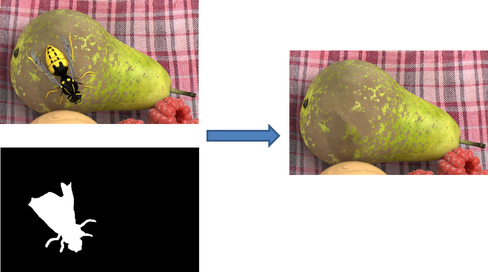
The goal of the proposed method is to consistently propagate the inpainting of one light
field view (e.g. the central view) to the rest of the light field by means of low rank matrix completion. The first step is then of inpainting one view (e.g. the central view) using any 2D image inpainting method.
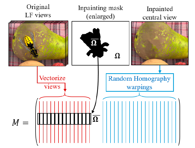
The consistent propagation of the inpainting through the entire light field is based on the premise that the views are highly correlated. As a consequence, the matrix formed by vectorizing each view and by concatenating the resulting column vectors, can be assumed to have a low rank (with respect to the number of views). Here, a line of the matrix contains the pixels values in all the views at a fixed (x,y) coordinate. Unfortunately, when the area to be removed has roughly the same position in all the views, many lines of the matrix only contain one known entry, corresponding to the central view. In this configuration, low rank completion is not able to recover reliably the unknown entries. Thus, in a preliminary step, we generate several additional views by warping the inpainted central view with a set of homography projections, and we insert the warped views in columns of the matrix to be completed as shown below.
Instead of computing
the homographies that globally compensate for the disparities
between the central view and the other views, we prefer
to generate a set of random homographies. This approach
allows a more uniform sampling of all the possible displacements
of each region of the image.
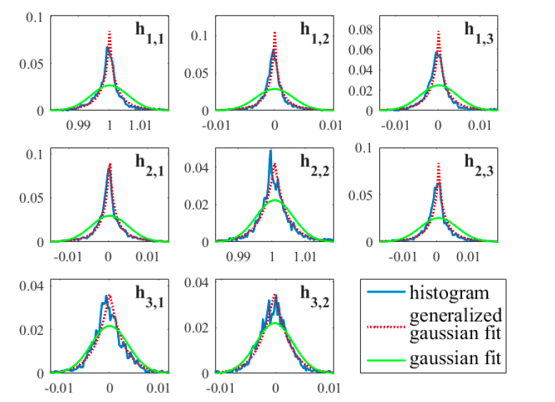
Eight parameters are
needed to determine one homography. In our method, we
need to carefully generate those values so that the resulting
homographies are within a reasonable range of rotation angle,
translation, shear etc. In order to determine a suitable
probability distribution function (pdf) for the eight parameters,
we have built a dataset of homographies from a set of
62 light field images captured with a Lytro camera. For all
the images, we have matched one homography between the
central view and each of the other views.
We have computed the marginal distributions of all the homography
parameters for our dataset.
We observe that the
eight distributions have a narrow peak around the mean
that is better modeled by a generalized gaussian distribution
(GGD) than a simple gaussian distribution. In order to
take into account the dependencies between the parameters,
we fit a multivariate GGD (MGGD) to the data. Random homography
parameters are then generated randomly using the known distribution.
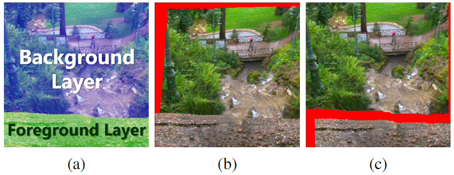
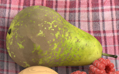
In the case where the area to recover contains several layers with different depth, the method can be improved by providing additionally a segmentation map of the different depth layers of the inpainted central view. This information is used by warping the layers with different homographies that are chosen randomly with the same MGGD distribution. The figure below shows two examples of random warpings in (b) and (c) obtained when a segmentation between a foreground and background layer is given for the inpainted central view (a). The areas shown in red are unknwon (e.g. occlusions, borders of the image), and are excluded from \(\Omega\) to be filled jointly with the original views by the low rank completion algorithm.
The consistent propagation of the inpainting through the entire light field is based on the premise that the views are highly correlated. As a consequence, the matrix formed by vectorizing each view and by concatenating the resulting column vectors, can be assumed to have a low rank (with respect to the number of views). Here, a line of the matrix contains the pixels values in all the views at a fixed (x,y) coordinate. Unfortunately, when the area to be removed has roughly the same position in all the views, many lines of the matrix only contain one known entry, corresponding to the central view. In this configuration, low rank completion is not able to recover reliably the unknown entries. Thus, in a preliminary step, we generate several additional views by warping the inpainted central view with a set of homography projections, and we insert the warped views in columns of the matrix to be completed as shown below.
 |
 |
In the case where the area to recover contains several layers with different depth, the method can be improved by providing additionally a segmentation map of the different depth layers of the inpainted central view. This information is used by warping the layers with different homographies that are chosen randomly with the same MGGD distribution. The figure below shows two examples of random warpings in (b) and (c) obtained when a segmentation between a foreground and background layer is given for the inpainted central view (a). The areas shown in red are unknwon (e.g. occlusions, borders of the image), and are excluded from \(\Omega\) to be filled jointly with the original views by the low rank completion algorithm.
 |
Inpainting Results
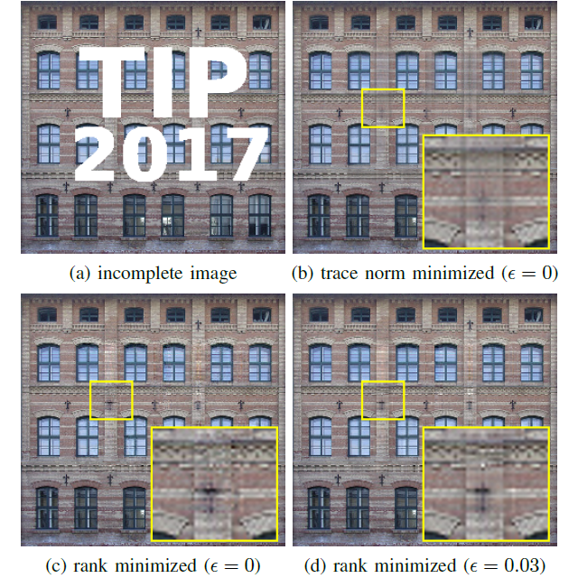
Evaluation of the proposed low rank matrix completion
The figure below shows the results obtained using either soft or hard thresholding for matrix completion in a simple 2D inpainting example. Sharper details are recovered
in the (c) and (d) sub-figures (hard thresholding), than in the (b) sub-figure (soft thresholding). In addition, we can observe in (d) that the introduction of the tolerance parameter (epsilon) successfully removes noise in the inpainted area.
 |
Inpainting results
Playing the inpainted light field as a video ro check the inter-view coherency of the inpainted region.
To play the video click on the image | 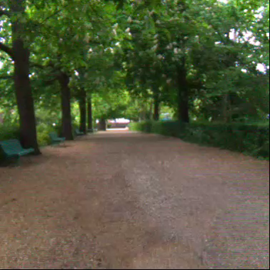
To play the video click on the image | 
To play the video click on the image |
|---|